Matrix Formalism

Detlef Smilgies

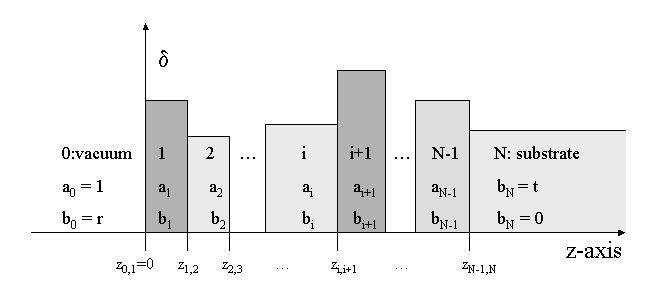
A typical application of a reflectivity measurement is, if we have a thin film on a substrate. Now we have to deal with two interfaces, air-film and film-substrate. We expect that the reflected wave from both interfaces interfere with each other and give rise to Kiessig fringes, from which the thickness of the film can be determined with high precision. We will treat the most general case now where we have n interfaces and the goal is, to understand how to solve the system of 2N boundary conditions.

Within each region i we have a wave vector k_z,i as given by the local index of refraction, and amplitudes a_i and b_i of the incident and the reflected waves, respectively. For the interface between layer i and layer i+1 at a distance z_i,i+1 from the top surface at z_0,1=0 and wave vectors k_z,i+1 and k_z,i on either side of the boundary, we get the following boundary condition for the wave amplitudes:

a_i exp(i k_z,i z_i,i+1) + b_i exp(-i k_z,i z_i,i+1) = a_i+1 exp(i k_z,i+1 z_i,i+1) + b_i+1exp(-i k_z,i+1 z_i,i+1)
k_z,i a_i exp(i k_z,i z_i,i+1) - k_z,i b_i exp(-i k_z,i z_i,i+1) = k_z,i+1 a_i+1 exp(i k_z,i+1 z_i,i+1) - k_z,i+1 b_i+1 exp(-i k_z,i+1 z_i,i+1)

and with some re-arranging

a_i = A_i,i+1,11 a_i+1 + A_i,i+1,12 b_i+1
b_i = A_i,i+1,21 a_i+1 + A_i,i+1,22 b_i+1

i.e. the transfer matrix A_i,i+1 relates the fields on either side of the interface i,i+1.

homework: calculate the components of the 2×2 matrix A_i,i+1

For the whole stack of N layers we thus get

(a₀, b₀) = A_0,1 A_1,2 ... A_i,i+1 ... A_N-1,N (a_N, b_N) = A (a_N, b_N)

a₀,b₀ and a_N,b_N are special: a₀ is just the incident wave onto the sample, b₀ yields the reflectivity signal we
observe:

a₀ = 1
b₀ = r

We assume an infinitely thick substrate, so there is no reflected wave in layer N:

b_N = 0

and a_N is the transmitted wave into the substrate. Hence we arrive at

(1, r) = A (t, 0)

which can be easily solved now for r and t

t = 1 / A₁₁
r = A₂₁ / A₁₁

We see that the general case involves more or less the same amount of calculation as the special cases of one or two layers. The outlined algorithm is known as the "matrix method" and is the algorithm mostly used these days.

History: Parratt at Cornell devised a similar algorithm [L.G. Parratt, Phys. Rev. B95, 359 (1954)] , which became very popular, in connection with Parrat's seminal papers on experimental applications of reflectivity. The matrix method is actually a couple of years older than Parratt's algorithm and was first published by F. Abelès [Ann. Physique (Paris) 5, 596 (1950)]. Similar schemes were already known in visible optics and spectroscopy - I know of an example in Max Born, Optik (1924), the predecessor of the classic optics book by Born and Wolf.

Note, that the matrix formalism has a direct analogon in quantum mechanics, namely reflection and transmission of a particle wave at a potential step or barrier (tunnel effect!). The requirement of continuity of the wave function ψ and its derivative at the potential step gives rise to the same boundary conditions as above. With respect to application in scattering, the quantum mechanical case is of importance for reflectivity studies with neutron beams.